Using the API#
The third and most flexible way to use yet_another_wizz is through its python API. Here we follow exactly the previous example and produce the same clustering redshift estimate.
The first step is to import the python package:
>>> import yaw
Loading the data#
All input data must be loaded as data catalogs, which can be done through the
NewCatalog factory class:
>>> factory = yaw.NewCatalog()
Next we load the reference sample. We want to split the data 32
spatial patches that allow us later to get uncertainties for our
clustering redshift measurements. By default these are generated automatically
with a k-means clustering algorithm when passing an integer to patches:
>>> reference = factory.from_file(
...     "reference.fits", ra="ra", dec="dec", redshift="z", patches=32)
>>> reference
ScipyCatalog(loaded=True, nobjects=389596, npatches=32, redshifts=True)
Now we can load the remaining catalogs. It is necessary that all catalogs use
exactly the same patch centers, which we directly assign from the reference
catalog using the patches parameter:
>>> randoms = factory.from_file(
...     "ref_rand.fits", patches=reference, ra="ra", dec="dec", redshift="z")
>>> unknown = factory.from_file(
...     "unknown.fits",  patches=reference, ra="ra", dec="dec")
Measuring correlations#
Next we construct a central Configuration object that sets
the minimal required parameters, the physical scales (in kpc)and the redshift
binning that we want to use for the correlation measurements:
>>> config = yaw.Configuration.create(rmin=100, rmax=1000, zmin=0.07, zmax=1.42)
Then we measure the correlation amplitudes using the
crosscorrelate() and
autocorrelate() functions. The latter allows to correct
for the reference sample galaxy bias:
>>> w_sp = yaw.crosscorrelate(config, reference, unknown, ref_rand=randoms)
>>> w_ss = yaw.autocorrelate(config, reference, randoms, compute_rr=True)
>>> w_ss
CorrFunc(n_bins=30, z='0.070...1.420', dd=True, dr=True, rd=False, rr=True, n_patches=32)
By inspecting the result we can see that this produced a
CorrFunc object with the desired binning and pair
counts data-data, data-random and random-random.
Getting the clustering redshifts#
Finally we can obtain our reference-sample-bias corrected clustering redshfit
estimate with a single line using the RedshiftData
container:
>>> n_cc = yaw.RedshiftData.from_corrfuncs(w_sp, w_ss)
>>> n_cc
RedshiftData(n_bins=30, z='0.070...1.420', n_samples=32, method='jackknife')
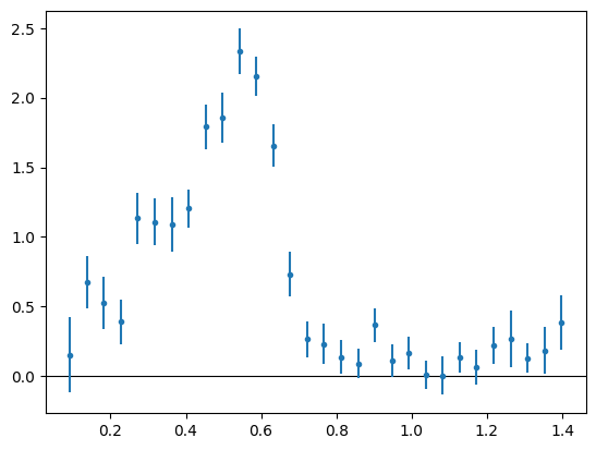
This object contains the redshift data and an error and covariance estimate computed from 32 jackknife realisations, based on the 32 spatial patches we created earlier. We can get a preview by using the builting plotting method:
>>> n_cc.plot(zero_line=True)
Storing the outputs#
Finally we can save those outputs to disk and reload them as needed, e.g.:
>>> w_ss.to_file("w_ss.hdf5")
>>> w_ss.from_file("w_ss.hdf5")
CorrFunc(n_bins=30, z='0.070...1.420', dd=True, dr=True, rd=False, rr=True, n_patches=32)
>>> n_cc.to_files("n_cc")
>>> n_cc.from_files("n_cc")
RedshiftData(n_bins=30, z='0.070...1.420', n_samples=32, method='jackknife')
For the latter we did not give a file extension, because the redshift data is stored in three separate files, one for the data and redshift estimate, one for the jackknife/bootstrap samples and one for the covariance matrix.
$ ls
n_cc.cov
n_cc.dat
n_cc.smp
w_ss.hdf5