Computing the redshift estimate#

In the final step take the previously computed pair counts to transform them to a redshift estimate. The code samples the correlation function and uses any provided sample autocorrelation function as a bias correction term for the measured cross-correlation:

ncc = yaw.RedshiftData.from_corrfuncs(
    cross_corr=cts_sp,
    ref_corr=cts_ss,
    # unk_corr=None,
)

This special RedshiftData object bundles the measured redshift estimate, its uncertainty, jackknife samples, and a covariance matrix estimate:

ncc.data  # length num_bins
ncc.error  # length num_bins
ncc.samples  # shape (num_samples=num_patches, num_bins)
ncc.covariance  # shape (num_bins, num_bins)

Similar to the pair counts, redshift estimates can be stored easily on disk, however as three separate human-readable text files.

ncc.to_files("nz_estimate")
    # data/error         ->  nz_estimate.dat
    # jackknife samples  ->  nz_estimate.smp
    # covariance         ->  nz_estimate.cov
# restored = yaw.RedshiftData.from_files("nz_estimate")

Additionally, the redshift estimate can be plotted easily:

ncc.plot(
    # label=None,
    # ax=None,  # plot to specific matplotlib axis
    # ...
)

# or even with estimated normalisation
ncc.normalised().plot()

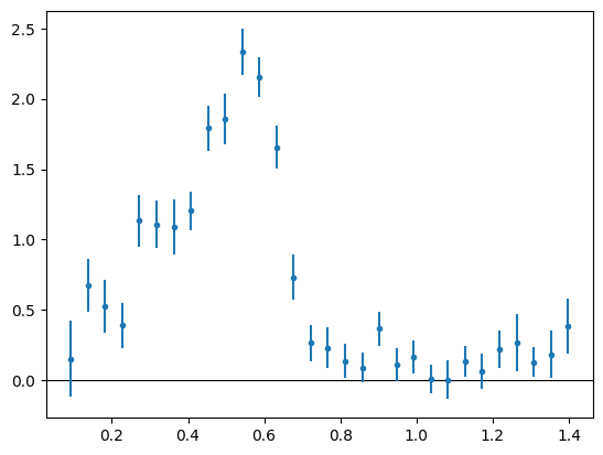
Example redshift estiamte — Example for the automatic plot of the final redshift estimate obtained from small test samples.#